In seismic data analysis a lot of work goes towards getting a good velocity model of the subsurface.
We talk about the seismic velocity. However, this may lead to some serious misconceptions.
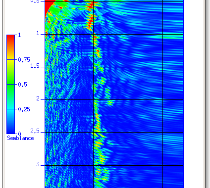
One step in seismic processing is velocity analysis. We pick the velocity that adjusts our data for the best value. Usually this is a quite colorful process, as you can see on the image:
This image shows which velocity will maximize the local energy over the total energy. This velocity is our so-called stacking velocity or also called normal moveout velocity. Initially, these may sound a little weird, but it’s not that hard actually. The normal moveout or NMO is the delay of arriving reflected energy when we increase the source-receiver distance (called offset). As long as the location of the source and the receiver are coincident, the path of the reflected energy is straight to the reflector and back up to the receiver.
However, due to the set-up of our seismic experiment, the illumination of a certain reflector will be done with varying source and receiver locations and hence varying offset. Unfortunately, this normal moveout is a non-linear stretch of the traces. This stretch can be corrected for by picking the right apparent velocity of the subsurface. Nevertheless, the velocity we picked is not even close to the real velocity as a rock property.
Stacking velocity and Inversion
The stacking velocity is a tool.
Stacking is the process of building a combined image of redundant data. In the most basic case this is a simple sum of the energy of our seismic traces.
It’s simply used to minimize the error, when correcting our seismic traces. However, we can utilize a process called inversion to find the velocity intervals in our seismic data. The easiest process to do this is the Dix inversion. It can get as complicated as a Full Waveform inversion that will take up significant computing power.
![]()
Of course the use of a Dix inversion is very limited. It assumes homogenity of the subsurface and availability of RMS velocities, but it’s an inversion that can actually be done with pen and paper.
What velocities are there actally?
We have a wide variety of velocities.
| Velocity | Usage |
|---|---|
| Vp vs. Vs | Velocities of longitudinally or transversally polarized waves. They’re the two types of body waves we usually look at. |
| Vnmo | The NMO velocity that corrects ideally for the NMO |
| Vrms | The Root Mean Square velocity. An average velocity of the different rocks. |
| Vstack | The stacking velocity minimizes the error of the stack |
| Vint | The interval velocity gives the velocity between two reflectors. Needed for migration; closest to an actual velocity. |
| Vmean | The mean velocity also differs from the other velocities. |
All of these velocities have a specific purpose in the seismic world, however these velocities have some very distinct limits as well.
These limits often include a phenomenon called anisotropy.### Anisotropy
In our everyday world we are used to things behaving isotropically. Even if you’ve never heard of isotropy, you are used to this concept. Every time you have a conversation with a friend, you may encounter communication problems but the sound waves travelling faster from one person to the other isn’t one of those. The speed of sound is equal in both directions.
Anisotropy is the opposite of isotropy. So to say the speed of sound is not the same into every direction anymore. You can compare this to taking an axe to hand for chopping wood for a fire. Personally, I prefer to put that log on the flat side take the axe to the opposite side. It’s pretty easy to get neat pieces in different sizes. If you were to put the log on the side and chop perpendicular to the direction of the fibres you will do a lot of chopping while others are already warming their fingers at a cozy fire. The wood does not behave equally in every direction. The resistance of the material is strong in a particular direction. This is something waves encounter in the subsurface as well. The seismic wave may have a harder time travelling into a certain direction compared to another one.
Anisotropy is a nuisance.
~ Helbig
When we look at our velocities in an anisotropic subsurface we may observe that it’s not possible anymore to differentiate between P- and S-waves. The polarization of these two wave types is only valid in isotropic media, so this has to be accounted for in seismic processing.
Group Velocity vs. Phase velocity
Until you learn about anisotropy in geophysics, you really don’t have to know the difference between group and phase velocity. That’s one of the reasons some geophysicists weren’t to psyched when anisotropy got important in data processing.Actually, seismologists have had to deal with this all the time, but seismics could escape these phenomenae until then.
We do seismics to extract data from the subsurface and this can only be done with a wave packet containing different frequencies. Then, it’s possible to “modulate” the wave, which is a psysicists way of saying that the wave behaves like a wave, with amplitude changes, phase shifts and most importantly the ability to carry signal information.
These different waves with differnt frequencies undergoing modulation can be seen as a group with a united group velocity. This group velocity sometimes seems a little abstract, but we have a mathematical trick to actually visualize this wave group. In the end we just have to draw a line that will include all the different phases with their according amplitudes. This is called an envelope.
Of course, it does not just end there. The heading already gave it away, we also have a phase velocity. Well, not quite, we have several. Every phase travels with its own velocity. I find this a bit hard to grasp, but the following gif portrays this pretty good.
In our subsurface we can readily assume that the group velocity is the one that carries the energy of the wave as well as the signal. However, when physicists get fancy, you cannot assume this on a general basis, as they have managed to construct a medium where the group velocity surpassed the speed of light, however information was still transmitted at a rate below the speed of light.Nemirovsky, J., Rechtsman, M., & Segev, M. (2012). Negative radiation pressure and negative effective refractive index via dielectric birefringence Optics Express, 20 (8) DOI: 10.1364/OE.20.008907
The big difference between the group and phase velocity can also be conveyed in their equations:
![]()
vs.
![]()
In a dispersive subsurface, this will cause a wave packet to stretch out over time. This stretch occurs due to the introduction of frequency dependence into the velocities. The effect may be a shift of lower frequencies to the back of the signal and higher frequencies to the front. This is called an up-chirped signal. However, in theory a medium in the subsurface could also have a negative group delay dispersion parameter that would cause lower frequencies to be faster than higher frequencies causing a down-chirp.
Quasi waves
As if this group velocity dispersion wasn’t enough, anisotropy has another effect on our seismic velocities.
When you look close enough at the equations that show the polarization of our P and S waves, there is a huge assumption of isotropy rearing its head. Once anisotropy is thrown into the mix, it gets tricky. The polarization in an isotropic medium is P, Sh and Sv, whereas Sh and Sv can be chosen arbitrarily. With anisotropy the polarizations aren’t that clear anymore. In the beginning stages of research into anisotropy people realized that the “P wave” now also includes a transversal polarization and the “S wave” has longitudinal parts. This renders the distinction between P and S waves utterly useless. However, geophysicists wouldn’t be a true physical discipline if we did not find a way to make nature fit our models and thinking. Hence, weak anisotropy was born. Under the assumption that our anisotropy “isn’t all that bad”, we can work with quasi P and quasi S waves, or short qP and qS.
What’s left?
In the end there is not one seismic velocity but many.
When we’re talking about seismic velocities it’s very context dependent and even without anisotropy it may be unclear. Always remember the quote of Helbig and make sure to know your velocity model very well. Seismic velocities depend a lot on the intended use. The first time you pick velocities with a professional tool you may see many many lines appearing as your velocity profile, have a look if you can identify them and learn something about your seismic data.
Jesper Dramsch
Latest posts by Jesper Dramsch (see all)
- Juneteenth 2020 - 2020-06-19
- All About Dashboards – Friday Faves - 2020-05-22
- Keeping Busy – Friday Faves - 2020-04-24